Checklist OAI 2026 Stage I · Task 1
Convolutional Filters
Polish title: Filtry konwolucyjne
Find one universal convolution kernel (at most 10×10) that restores corrupted photographs, and an upsampling method (plus optional kernel) that restores them from half resolution.
The task
The introduction explains images as grids of pixel values, convolution with a small kernel (with identity, blur, sharpen and vertical-edge examples) and nearest-neighbour upsampling. The task has two independently scored parts.
Part 1: find a single universal kernel, returned by compute_kernel(), that restores corrupted images as closely as possible to the originals; the kernel may be at most 10×10. The starter kernel is a 9×9 blur, and optimisation with PyTorch autograd is suggested.
Part 2: implement upsample(image), which enlarges a downsampled image of shape (C, h, w) to full size (C, H, W), and optionally compute_kernel_upsampling(kernel_task1), a kernel applied after upsampling (by default the Part 1 kernel). Nearest-neighbour upsampling is the reference baseline. Each example is a triple of the original 256×256 RGB image, its corrupted version (256×256) and the corrupted version downsampled to 128×128, as tensors with values in [0, 1].
Abridged and translated by SOTA from the official Polish materials. The official statement has the exact rules, and it wins wherever this summary differs.
In English
This task was published in Polish. SOTA translated it into English on 16 September 2026. Only the words changed in the notebooks: markdown, code comments, messages and printed output. The code, file names and paths are the original's, so a translated notebook runs with the original data.
Read the task notebook in English
Convolutional Filters
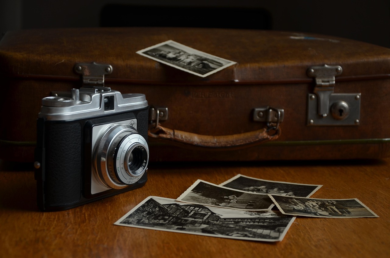
Source: Pixabay
Introduction
Imagine that you find some old family photographs in the attic. Unfortunately, the passage of time has left the photos faded, noisy and blurry. You want to restore them and bring back their former glory. You could spend many hours correcting them by hand in a graphics program, but what if it were possible to create a single, universal "magic filter" that automatically repairs every damaged photo?
In this task, your goal is precisely to create such a "recipe" for repairing images. In the world of computer science and artificial intelligence, this recipe is called a convolution kernel. It is a fundamental tool in image processing, and it underlies the way computers "see" and understand the world.
What is Convolution?
Before we move on to the task, we need to understand two things: what an image is to a computer, and how the "magic filter", that is, convolution, acts on it.
What is an image to a computer?
To us, an image is a face, a landscape or a cat. To a computer, it is simply a large grid of numbers. Each number in this grid corresponds to the brightness of one pixel. In colour images we have three such grids – one for red (R), one for green (G) and one for blue (B).
How does convolution work?
Convolution is an operation in which a small matrix of numbers (e.g. of size 3x3), called a kernel, is slid across the whole image, pixel by pixel.
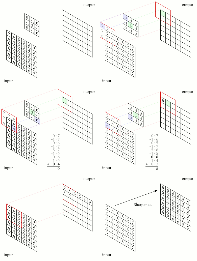
Source: Michael Plotke, CC BY-SA 3.0 https://creativecommons.org/licenses/by-sa/3.0, via Wikimedia Commons
For each position of the kernel on the image, we perform a simple operation:
- We take the fragment of the image lying under the kernel and multiply the corresponding pixel values and kernel weights.
- We sum all of these results.
- The result of this sum becomes the new pixel value in the new, processed image.
Depending on which numbers we put into the kernel, we obtain completely different effects.
Examples of kernels
| Kernel (3x3 matrix) | Effect on the image |
|---|---|
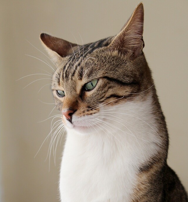
| Identity The one in the centre makes the new pixel an exact copy of the original one. $$\begin{bmatrix} 0 & 0 & 0 \ 0 & 1 & 0 \ 0 & 0 & 0 \end{bmatrix}$$ |
 |
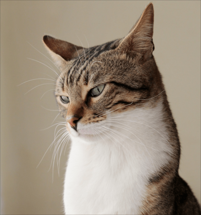
| Blurring Averages the value of a pixel with its neighbours, which smooths the image. $$\begin{bmatrix} \frac{1}{9} & \frac{1}{9} & \frac{1}{9} \ \frac{1}{9} & \frac{1}{9} & \frac{1}{9} \ \frac{1}{9} & \frac{1}{9} & \frac{1}{9} \end{bmatrix}$$ |
 |
| Sharpening Emphasises the differences between a pixel and its surroundings, bringing out details. $$\begin{bmatrix} 0 & -1 & 0 \ -1 & 5 & -1 \ 0 & -1 & 0 \end{bmatrix}$$ |
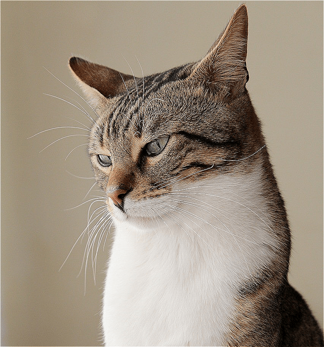 |
| Vertical edge detection Strengthens places where there are dark pixels on the left and bright pixels on the right. $$\begin{bmatrix} -1 & 0 & 1 \ -2 & 0 & 2 \ -1 & 0 & 1 \end{bmatrix}$$ |
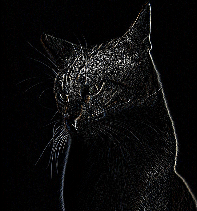 |
And what is upsampling?
In the second part of the task, you will encounter the concept of upsampling, that is, enlarging an image. It is the reverse of reducing an image (downsampling): we have a small image, e.g. 128x128 pixels, and we want to obtain a larger one from it — e.g. 256x256.
The problem is that the computer does not know what the values of the new, "invented" pixels should be. That is why it has to guess them somehow.
The simplest way is to come up with a very simple rule, for example the following one (called nearest neighbor upsampling):
Each pixel of the small image is simply replicated horizontally and vertically as many times as needed to fill a larger block of pixels.
As a result, the enlarged image looks like an enlarged "mosaic" — the shapes are preserved, but sharp edges and large pixels are clearly visible.
Task
In this task, you will work on two related parts:
- Part one — Convolutional kernel
- Part two — Upsampling (enlarging images)
Each of them is scored independently.
Part 1 — Convolutional kernel
Your task is to find a single, universal kernel (filter) that can restore damaged photos to a form as close as possible to the originals.
Note: The size of the kernel should not exceed 10x10.
As a starting point, you are given the function compute_kernel(),
which returns a simple filter — a so-called 9x9 blurring kernel (above you will find an example showing how such a kernel works at a size of 3x3).
Instead of choosing the weights by hand, you can use the autograd mechanism from the PyTorch library. It is used for automatic optimisation – in an iterative process, it will adjust the values in the kernel so that the image reconstruction error is as small as possible.
Part 2 — Upsampling
In the second part, you will focus on the problem of enlarging images.
This time, your task is to implement the function upsample(image: torch.Tensor) -> torch.Tensor,
which receives a downscaled image ((C, h, w)) and has to enlarge it to full size ((C, H, W)).
The reference point (baseline) will be a very simple method, nearest neighbor, which replicates each pixel the appropriate number of times vertically and horizontally.
In addition to the upsample function, you can also choose an additional kernel (computed by the function compute_kernel_upsampling(kernel_task1: torch.Tensor) -> torch.Tensor), which will be applied after upsampling, on the already enlarged image. By default, this is the kernel from the first part of the task.
In this part, the quality of the image reconstruction is scored after two steps:
- upsampling (the
upsample()function), - convolution with your kernel (the
compute_kernel_upsampling(...)function).
Data
In this task, two datasets saved in a single file (train_val.npz) are available to you:
train_ds— 150 training examples,val_ds— 50 validation examples.
Each example is a triple of related images:
image_original– the original, correct image at a resolution of 256x256 pixels,image_corrupted– the same image after distortion, also 256x256,image_corrupted_downsampled– a version ofimage_corrupteddownscaled to 128x128, on which you will test your upsampling methods.
All images are in colour (RGB) and are stored as PyTorch tensors of shape (3, H, W)
with values normalised to the range [0, 1].
Scoring Criterion
Both parts of the task will be scored using the MSE (Mean Squared Error) metric. It is a simple way of measuring how much two images differ from each other. The metric computes the difference between each pixel in the reconstructed image and in the original one, squares these differences and takes their mean.
The lower the MSE value, the more similar the images are to each other, and the better your solution is.
Part 1 (70 pts) - Convolutional kernel
- For this part you can earn a maximum of 70 points.
- If the MSE value for your solution is 0.0285 (or more), you will receive 0 points for this part of the task.
- If the MSE value for your solution is 0.0077 (or less), you will receive 70 points for this part of the task.
- Otherwise, the number of points will be determined in proportion to the MSE value:
Part 2 (30 pts) - Upsampling
- For this part you can earn a maximum of 30 points.
- If the MSE value for your solution is 0.0542 (or more), you will receive 0 points for this part of the task.
- If the MSE value for your solution is 0.0350 (or less), you will receive 30 points for this part of the task.
- Otherwise, the number of points will be determined in proportion to the MSE value:
Final score
The final score is the sum of the scores for both parts:
that is:
- 70% of the points come from the quality of your kernel (the
compute_kernel()function) - 30% of the points come from the quality of your
upsample()andcompute_kernel_upsampling()functions.
Constraints
- Your solution will be tested on the Contest Platform without Internet access, in an environment with a GPU.
- The evaluation of your final solution on the Contest Platform must not take longer than 3.5 minutes with a GPU.
- Permitted libraries:
numpy,torch(thetorch.nnmodule may not be used in the solution).
Submission Files
This notebook, completed with your solution (the functions compute_kernel, compute_kernel_upsampling and upsample).
Evaluation
Remember that during grading the FINAL_EVALUATION_MODE flag will be set to True.
For this task you can earn between 0 and 100 points. The number of points you earn will be calculated on the (secret) test set on the Contest Platform using the formula given above, rounded to an integer. If your solution does not meet the criteria above or does not run correctly, you will receive 0 points for the task.
Starter Code
In this section we initialise the environment by importing the required libraries and functions. The code provided will make it easier for you to work with the data efficiently and to build your solution.
######################### DO NOT CHANGE THIS CELL ###########################

FINAL_EVALUATION_MODE = False  # We will set this flag to True during grading.
######################### DO NOT CHANGE THIS CELL ###########################
if not FINAL_EVALUATION_MODE:
import matplotlib.pyplot as plt
import os
import torch
import numpy as np
import math
import shutil
from typing import Callable, Optional
DEVICE = torch.device("cuda" if torch.cuda.is_available() else "cpu")######################### DO NOT CHANGE THIS CELL ###########################
seed = 12345
os.environ["PYTHONHASHSEED"] = str(seed)
torch.manual_seed(seed)
torch.backends.cudnn.deterministic = True
torch.backends.cudnn.benchmark = False######################### DO NOT CHANGE THIS CELL ###########################
# Cell containing helper functions for preparing the data.
def download_data() -> None:
"""Downloads the dataset from Google Drive and saves it in the 'data' folder."""
import gdown
# Create or reset the 'data' folder
if not os.path.exists('data'):
os.makedirs('data')
else:
shutil.rmtree('data')
os.makedirs('data')
# Download the file from Google Drive and save it in the 'data' folder
url = "https://drive.google.com/file/d/1wzYqBQ56IMXpM7_gv05vzercvZSZy-Ps/view?usp=drive_link"
output = f'data/train_val.npz'
gdown.download(url, output, quiet=True, fuzzy=True)
def setup_data_from_npz(npz_path: str) -> tuple[list[dict], list[dict]]:
"""
Loads triples of images (original, corrupted and downscaled (downsampled)
corrupted) from an NPZ file and returns them as two lists of dictionaries.
Args:
npz_path (str): Path to the .npz file with the data.
Returns:
tuple[list[dict], list[dict]]:
- train_ds: a list of dictionaries {'image_original': tensor,
'image_corrupted': tensor, 'image_corrupted_downsampled': tensor}
- val_ds: a list of dictionaries in the same format, but for validation.
"""
# Loading the data from the file
data = np.load(npz_path, allow_pickle=True)
train_list = data['train_ds'].tolist()
val_list = data['val_ds'].tolist()
def to_tensor_triplet(sample: dict) -> dict:
# We convert the loaded data (uint8) to float32
# and scale it back to the range [0, 1] by dividing by 255.0
return {
"image_original": torch.from_numpy(sample["image_original"]).to(torch.float32) / 255.0,
"image_corrupted": torch.from_numpy(sample["image_corrupted"]).to(torch.float32) / 255.0,
"image_corrupted_downsampled": torch.from_numpy(sample["image_corrupted_downsampled"]).to(torch.float32) / 255.0,
}
train_ds = [to_tensor_triplet(s) for s in train_list]
val_ds = [to_tensor_triplet(s) for s in val_list]
return train_ds, val_ds######################### DO NOT CHANGE THIS CELL ###########################
# Cell containing helper functions for evaluating the solution.
def _pad_replicate(x: torch.Tensor, pad: int) -> torch.Tensor:
"""
"Padding by replication" — adds a border made of the image's edge pixels.
Useful for convolution operations (the kernel is in the centre, the edge does not "escape").
Args:
x (torch.Tensor): Image of shape (C, H, W).
pad (int): Number of pixels to add on each side.
Returns:
torch.Tensor: Image of enlarged size (C, H+2*pad, W+2*pad).
"""
if pad == 0:
return x
# Vertical padding: we duplicate the first and the last row.
top = x[:, :1, :].expand(-1, pad, -1)
bottom = x[:, -1:, :].expand(-1, pad, -1)
xvb = torch.cat([top, x, bottom], dim=1) # (C, H+2p, W)
# Horizontal padding: we duplicate the first and the last column.
left = xvb[:, :, :1].expand(-1, -1, pad)
right = xvb[:, :, -1:].expand(-1, -1, pad)
xpad = torch.cat([left, xvb, right], dim=2) # (C, H+2p, W+2p)
return xpad
def apply_kernel(image: torch.Tensor, kernel: torch.Tensor) -> torch.Tensor:
"""
Applies the same filter (kernel) to each channel component of the image.
Args:
image (torch.Tensor): Image of shape (C, H, W) in the range [0,1].
kernel (torch.Tensor): 2D filter of shape (K, K).
Returns:
torch.Tensor: New image (C, H, W) after applying the kernel.
"""
assert image.dim() == 3, "image must have dimensions (C,H,W)"
assert kernel.dim() == 2 and kernel.size(0) == kernel.size(1), "kernel must be a square (K,K)"
assert kernel.size(0) <= 10, "the kernel size must not exceed 10x10"
C, H, W = image.shape
K = kernel.size(0)
pad = K // 2
# Padding by replication (without in-place modification — important for autograd).
xpad = _pad_replicate(image, pad) # (C, H+2p, W+2p)
# We create "windows" of neighbouring pixels for each location in the image: (C, H, W, K, K)
sC, sH, sW = xpad.stride()
windows = xpad.as_strided(
size=(C, H, W, K, K),
stride=(sC, sH, sW, sH, sW)
)
# We compute the correlation: element-wise multiplication and summation over the KxK neighbourhood
out = (windows * kernel.view(1, 1, 1, K, K)).sum(dim=(-1, -2)) # (C,H,W)
return out
def evaluate_solution(
kernel: torch.Tensor,
ds: list[dict],
upsample_fun: Optional[Callable] = None
) -> float:
"""
Computes the mean MSE (Mean Squared Error) on the given dataset.
Args:
kernel (torch.Tensor): 2D filter (e.g. 5x5) to be evaluated.
ds (list[dict]): List of samples with the keys 'image_original',
'image_corrupted' and 'image_corrupted_downsampled'.
upsample_fun (Optional[Callable]): (Optional) Upsampling function
(torch.Tensor -> torch.Tensor) to be evaluated.
Returns:
float: Mean MSE value for the whole set.
"""
total_mse = 0.0
kernel = kernel.to(DEVICE)
# We do not need gradients during evaluation — this speeds things up and saves memory.
with torch.no_grad():
for sample in ds:
original = sample['image_original'].to(DEVICE)
# Choosing the appropriate "corrupted" version:
# - if an upsampling function is given, we enlarge the downscaled version,
# - otherwise we take the full-size version.
if upsample_fun is not None:
corrupted = sample['image_corrupted_downsampled'].to(DEVICE)
corrupted = upsample_fun(corrupted) # we expect (C, H, W)
else:
corrupted = sample['image_corrupted'].to(DEVICE) # already (C, H, W)
# Reconstructing the image by applying the kernel to the "corrupted" image.
reconstructed = apply_kernel(corrupted, kernel)
# MSE: the mean of the squared pixel-by-pixel differences.
mse = torch.mean((reconstructed - original)**2)
total_mse += mse.item()
return total_mse / len(ds)
def round_half_up(number: float) -> int:
"""
Rounds to the nearest integer (.5 always rounds up).
"""
return int(math.floor(number + 0.5))
def compute_score(kernel_mse: float, upsampling_mse: float) -> tuple[int, int, int]:
"""
Converts the two MSE results (for the kernel and for upsampling) into a single score of 0–100.
Each MSE is mapped separately onto a point scale based on thresholds,
and the results are then combined using weights.
Args:
kernel_mse (float): Mean MSE for part 1 (kernel).
upsampling_mse (float): Mean MSE for part 2 (upsampling).
Returns:
tuple[int, int, int]: A tuple containing the final score (0–100),
the score for part 1 (kernel) and the score for part 2 (upsampling).
"""
# Quality thresholds: the lower the MSE, the better.
# 100 pts are awarded for MSE <= lower_bound,
# 0 pts for MSE >= upper_bound,
# otherwise — between 100 and 0 (the score is scaled linearly).
KERNEL_LOWER = 0.0077
KERNEL_UPPER = 0.0285
UPS_LOWER = 0.0350
UPS_UPPER = 0.0542
# Weights of the parts of the task.
KERNEL_W = 0.7
UPS_W = 0.3
def linear_score(mse: float, lower: float, upper: float) -> float:
"""
Maps the MSE onto the interval [0,100] according to the thresholds.
- mse <= lower -> 100
- mse >= upper -> 0
- in between -> linearly between 100 and 0
"""
if mse <= lower:
return 100.0
if mse >= upper:
return 0.0
# the closer to lower, the more points
return 100.0 * (upper - mse) / (upper - lower)
kernel_score = round_half_up(KERNEL_W * linear_score(kernel_mse, KERNEL_LOWER, KERNEL_UPPER))
upsampling_score = round_half_up(UPS_W * linear_score(upsampling_mse, UPS_LOWER, UPS_UPPER))
# We combine the scores and clip the total to [0,100] just in case.
final_score = kernel_score + upsampling_score
final_score = max(0, min(100, final_score))
return final_score, kernel_score, upsampling_score######################### DO NOT CHANGE THIS CELL ###########################
# Cell containing helper functions for visualisation.
def plot_results(
original: torch.Tensor,
corrupted: torch.Tensor,
reconstructed: torch.Tensor,
title: str = "Reconstruction results",
labels: tuple = ("Original", "Corrupted", "Reconstructed"),
center_smaller: bool = True,
background: float = 1.0,
show_shapes: bool = True,
clip_for_display: bool = True
) -> None:
"""
Displays three images side by side. If one of the images is smaller
than the largest of the others and `center_smaller=True`, it is only
**centred** on a canvas the size of the largest image (by means of
padding with the background colour), so that the panel sizes are visually consistent.
Args:
original (torch.Tensor): Reference image in (C, H, W) format, values in [0, 1].
corrupted (torch.Tensor): "Corrupted" image in (C, h, w) format; it may be smaller.
reconstructed (torch.Tensor): Image after reconstruction in (C, H, W) format.
title (str): Title of the whole figure.
labels (tuple): Captions above the panels (from the left): ("Original", "Corrupted", "Reconstructed").
center_smaller (bool): If True, smaller images are centred with padding (without scaling).
background (float): Background (padding) colour in [0, 1]; 1.0 = white, 0.0 = black.
show_shapes (bool): If True, the sizes (height×width) are appended to the panel titles.
clip_for_display (bool): If True, clips only a copy of the data to [0,1]
for imshow (eliminates warnings and "burnt-out" areas on screen).
Returns:
None
"""
import numpy as np
def to_hwc_np(t: torch.Tensor) -> np.ndarray:
"""
Converts a (C, H, W) tensor into a NumPy array (H, W, C) in [0, 1],
without modifying the values.
"""
return t.detach().cpu().permute(1, 2, 0).numpy()
def pad_center(img_hwc: np.ndarray, target_hw: tuple, bg: float) -> np.ndarray:
"""
Pastes an image (H, W, C) into the centre of a canvas of size target_hw (H_t, W_t).
Args:
img_hwc (np.ndarray): Input image (H, W, C) in [0, 1].
target_hw (tuple[int,int]): Target canvas size (H_t, W_t).
bg (float): Background colour in [0, 1].
Returns:
np.ndarray: Image (H_t, W_t, C) with the input image centred.
"""
Ht, Wt = target_hw
h, w, c = img_hwc.shape
# If the sizes already match, or we do not want to centre, we return the image unchanged
if (h, w) == (Ht, Wt) or not center_smaller:
return img_hwc
# We create a background canvas and paste the image in the middle
canvas = np.full((Ht, Wt, c), bg, dtype=img_hwc.dtype)
top = (Ht - h) // 2
left = (Wt - w) // 2
canvas[top:top + h, left:left + w, :] = img_hwc
return canvas
# Conversion to HWC numpy
img_o = to_hwc_np(original)
img_c = to_hwc_np(corrupted)
img_r = to_hwc_np(reconstructed)
# Common frame = the maximum size among the inputs
Hs = [img_o.shape[0], img_c.shape[0], img_r.shape[0]]
Ws = [img_o.shape[1], img_c.shape[1], img_r.shape[1]]
target_hw = (max(Hs), max(Ws))
# Padding only if needed
img_o_pad = pad_center(img_o, target_hw, background)
img_c_pad = pad_center(img_c, target_hw, background)
img_r_pad = pad_center(img_r, target_hw, background)
# Optionally append the sizes to the titles
titles = list(labels)
if show_shapes:
titles[0] = f"{titles[0]} ({img_o.shape[0]}×{img_o.shape[1]})"
titles[1] = f"{titles[1]} ({img_c.shape[0]}×{img_c.shape[1]})"
titles[2] = f"{titles[2]} ({img_r.shape[0]}×{img_r.shape[1]})"
# Optional clipping for display only
if clip_for_display:
def clip01(a: np.ndarray) -> np.ndarray:
return np.clip(a, 0.0, 1.0, out=a.copy())
show_o = clip01(img_o_pad)
show_c = clip01(img_c_pad)
show_r = clip01(img_r_pad)
else:
show_o, show_c, show_r = img_o_pad, img_c_pad, img_r_pad
# Drawing
fig, axes = plt.subplots(1, 3, figsize=(15, 5))
for ax, img, lab in zip(axes, (show_o, show_c, show_r), titles):
ax.imshow(img, origin="upper")
ax.set_title(lab)
ax.axis("off")
fig.suptitle(title)
plt.tight_layout()
plt.show()Loading the Data
Using the code below, the data will be downloaded and prepared appropriately.
######################### DO NOT CHANGE THIS CELL ###########################

if not FINAL_EVALUATION_MODE:
    download_data()

    # Path to the single NPZ file with the data (training + validation)
    NPZ_PATH = os.path.join('data', 'train_val.npz')

    # Load the sets from the NPZ file
    train_ds, val_ds = setup_data_from_npz(NPZ_PATH) # These variables will also be available during the final evaluation

    if train_ds is not None and val_ds is not None:
        print(f"Number of images in the training set: {len(train_ds)}")
        print(f"Number of images in the validation set: {len(val_ds)}")

        # Preview of example data
        sample_for_show = val_ds[0]
        plot_results(sample_for_show['image_original'], sample_for_show['image_corrupted'], sample_for_show['image_corrupted_downsampled'], title="Example data from the NPZ file", labels=("Original", "Corrupted", "Corrupted (downsampled)"))
Your Solution
Below we present simplified solutions that serve as an example. These solutions achieve very poor results, but they demonstrate the answer format we expect and can serve as a starting point for your implementation.
Place your solution in this section. Make changes only here. The following functions will be passed on for evaluation:
compute_kernel() -> torch.Tensor,upsample(image: torch.Tensor) -> torch.Tensor,compute_kernel_upsampling(kernel_task1: torch.Tensor) -> torch.Tensor
Within them, you may call additional helper functions.
The previously prepared training and validation data are available in the variables train_ds, val_ds.
Part 1 - Convolutional kernel
def compute_kernel() -> torch.Tensor:
    """
    Creates a blurring kernel of size 9x9.
    """
    kernel = torch.ones(9, 9, device=DEVICE) / 81
    return kernel
Part 2 - Upsampling
def upsample(image: torch.Tensor) -> torch.Tensor:
    """
    Simple upsampling using the "nearest neighbour" method (nearest neighbor)
    to a size of 256x256.

    Idea:
    Each pixel of the smaller image is simply replicated several times
    vertically and horizontally. As a result, the image becomes larger, but no new
    details appear – we only see the "stretched" original pixels.

    Args:
        image (torch.Tensor): Image in (C, h, w) format, where:
            - C is the number of channels (e.g. 3 for RGB),
            - h, w are the height and width of the image (≤ 256).

    Returns:
        torch.Tensor: Image of shape (C, 256, 256) obtained by
        repeating the rows and columns of the input as many times as needed
        to cover the whole target size, and then cropping to the exact
        dimensions of 256x256.
    """
    assert image.dim() == 3, "Expecting a tensor of shape (C, h, w)."
    C, h, w = image.shape

    # Target dimensions.
    Ht, Wt = (256, 256)

    # How many times we must repeat the rows and columns to reach >= 256.
    rh = max(1, math.ceil(Ht / h))
    rw = max(1, math.ceil(Wt / w))

    # repeat_interleave replicates successive rows/columns the appropriate number of times.
    y = image.repeat_interleave(rh, dim=1).repeat_interleave(rw, dim=2)

    # It may happen that there are "too many" repetitions – in that case we crop to 256x256.
    return y[:, :Ht, :Wt]
def compute_kernel_upsampling(kernel_task1: torch.Tensor) -> torch.Tensor:
"""
During evaluation, the kernel from the first part will be passed
as an argument. You may use it or ignore it.
"""
return kernel_task1Evaluation
Running the cell below lets you check how many points your solution would earn on the validation data.
Before submitting, make sure that the whole notebook runs from start to finish without errors and without user intervention after executing the Run All command.
######################### DO NOT CHANGE THIS CELL ###########################

if not FINAL_EVALUATION_MODE:

    # ============== 1) First part of the task ==============
    # -- Training
    your_kernel = compute_kernel()
    # -- Evaluation of the solution
    your_kernel_mse = evaluate_solution(your_kernel, val_ds)

    # ============== 2) Second part of the task ==============
    # -- Training
    your_kernel_upsampling = compute_kernel_upsampling(your_kernel)
    # -- Evaluation of the solution
    your_upsampling_mse = evaluate_solution(your_kernel_upsampling, val_ds, upsample)

    score, kernel_score, upsampling_score = compute_score(your_kernel_mse, your_upsampling_mse)

    print(f"MSE on the validation set (kernel): {your_kernel_mse:.4f}. Number of points (kernel): {kernel_score}")
    print(f"MSE on the validation set (upsampling): {your_upsampling_mse:.4f}. Number of points (upsampling): {upsampling_score}")
    print(f"Estimated number of points for the task: {score}")

    # Visualisation of the effect of the kernel on a single validation image.
    sample_for_show = val_ds[0]
    reconstructed = apply_kernel(sample_for_show['image_corrupted'].to(DEVICE), your_kernel.to(DEVICE))
    plot_results(sample_for_show['image_original'], sample_for_show['image_corrupted'], reconstructed, title="Visualisation of the effect of your kernel")

    # Preview of the kernel itself (colour map).
    plt.figure(figsize=(5, 5))
    plt.imshow(your_kernel.cpu().detach().numpy(), cmap='viridis')
    plt.colorbar()
    plt.title("Your kernel")
    plt.show()

    # Visualisation of the effect of upsampling with the kernel on a single validation image.
    reconstructed = apply_kernel(upsample(sample_for_show['image_corrupted_downsampled'].to(DEVICE)), your_kernel_upsampling)
    plot_results(sample_for_show['image_original'], sample_for_show['image_corrupted_downsampled'], reconstructed, title="Visualisation of the effect of your upsampling method with the kernel", labels=("Original", "Corrupted (downsampled)", "Reconstructed"))
Translated by SOTA. The Polish original is the official version and wins wherever the two differ. The three large plot outputs from the original run are not included in the English copy; see the original notebook for them. If you organise this olympiad and would like the translation removed, email [email protected] and we will take it down.
At a glance
- You get
train_val.npzwithtrain_ds(150 examples) andval_ds(50 examples), downloaded from Google Drive.- You submit
- This notebook with
compute_kernel,compute_kernel_upsamplingand upsample. - Scoring
- MSE against the originals. Part 1 (70 points): round((0.0285 − MSE_kernel)/(0.0285 − 0.0077) × 70), 0 at MSE ≥ 0.0285 and 70 at MSE ≤ 0.0077. Part 2 (30 points): round((0.0542 − MSE_upsampling)/(0.0542 − 0.0350) × 30), 0 at MSE ≥ 0.0542 and 30 at MSE ≤ 0.0350. Final score is the sum.
- Rules
- Tested without Internet access, with a GPU; evaluation must take at most 3.5 minutes.
- Allowed libraries: numpy and torch; torch.nn may not be used in the solution.
- Kernel size at most 10×10.
- Format
- Stage I (online), 1 December 2025 – 25 January 2026; up to 100 points per task (500 in total; the qualification threshold for Stage II was 350 points). Tasks are ordered by intended increasing difficulty. Evaluated automatically on the Competition Platform (Platforma Konkursowa) on a hidden test set; points are rounded to an integer, and a notebook that fails the requirements or does not run scores 0.